broomの基本操作

library(tidyverse)
library(broom)

1 broomとは

broomパッケージは，回帰分析などの統計モデルの出力を整然としたデータフレーム（tibble）に変換するためのパッケージです．Rの標準的なsummary()関数の出力はリスト形式で扱いにくいことがありますが，broomを使えばtidyverseの流儀に沿ったデータ操作が可能になります．

broomには3つの主要な関数があります．

tidy()：モデルの係数や検定結果を整理する
glance()：モデル全体の適合度を要約する
augment()：元データに予測値や残差を追加する

2 準備：回帰分析の実行

まず，例として単回帰分析を実行します．

wagedata <- read_csv("wage.csv", show_col_types = FALSE)

model <- lm(wage ~ educ, data = wagedata)

summary()の出力は情報量が多いですが，プログラムで扱いにくい形式です．

summary(model)


Call:
lm(formula = wage ~ educ, data = wagedata)

Residuals:
    Min      1Q  Median      3Q     Max 
-576.09 -173.36  -34.12  127.82 1686.25 

Coefficients:
            Estimate Std. Error t value Pr(>|t|)    
(Intercept)  183.949     23.104   7.962 2.38e-15 ***
educ          29.655      1.708  17.368  < 2e-16 ***
---
Signif. codes:  0 '***' 0.001 '**' 0.01 '*' 0.05 '.' 0.1 ' ' 1

Residual standard error: 250.7 on 3008 degrees of freedom
Multiple R-squared:  0.09114,   Adjusted R-squared:  0.09084 
F-statistic: 301.6 on 1 and 3008 DF,  p-value: < 2.2e-16

3 `tidy()`：係数の整理

tidy()は，各係数の推定値，標準誤差，検定統計量，p値をtibbleとして返します．

tidy(model)

# A tibble: 2 × 5
  term        estimate std.error statistic  p.value
  <chr>          <dbl>     <dbl>     <dbl>    <dbl>
1 (Intercept)    184.      23.1       7.96 2.38e-15
2 educ            29.7      1.71     17.4  1.83e-64

パイプ演算子と組み合わせることもできます．

lm(wage ~ educ, data = wagedata) %>%
  tidy()

# A tibble: 2 × 5
  term        estimate std.error statistic  p.value
  <chr>          <dbl>     <dbl>     <dbl>    <dbl>
1 (Intercept)    184.      23.1       7.96 2.38e-15
2 educ            29.7      1.71     17.4  1.83e-64

conf.int = TRUEを指定すると，信頼区間も出力されます．

model %>%
  tidy(conf.int = TRUE)

# A tibble: 2 × 7
  term        estimate std.error statistic  p.value conf.low conf.high
  <chr>          <dbl>     <dbl>     <dbl>    <dbl>    <dbl>     <dbl>
1 (Intercept)    184.      23.1       7.96 2.38e-15    139.      229. 
2 educ            29.7      1.71     17.4  1.83e-64     26.3      33.0

信頼水準を変更するには，conf.levelを指定します．

model %>%
  tidy(conf.int = TRUE, conf.level = 0.99)

# A tibble: 2 × 7
  term        estimate std.error statistic  p.value conf.low conf.high
  <chr>          <dbl>     <dbl>     <dbl>    <dbl>    <dbl>     <dbl>
1 (Intercept)    184.      23.1       7.96 2.38e-15    124.      243. 
2 educ            29.7      1.71     17.4  1.83e-64     25.3      34.1

4 `glance()`：モデル全体の要約

glance()は，決定係数\(R^2\)やAICなど，モデル全体の適合度指標を1行のtibbleとして返します．

glance(model)

# A tibble: 1 × 12
  r.squared adj.r.squared sigma statistic  p.value    df  logLik    AIC    BIC
      <dbl>         <dbl> <dbl>     <dbl>    <dbl> <dbl>   <dbl>  <dbl>  <dbl>
1    0.0911        0.0908  251.      302. 1.83e-64     1 -20898. 41803. 41821.
# ℹ 3 more variables: deviance <dbl>, df.residual <int>, nobs <int>

5 `augment()`：予測値と残差の追加

augment()は，元のデータに予測値（.fitted）や残差（.resid）などの列を追加したtibbleを返します．

augment(model) %>%
  head()

# A tibble: 6 × 8
   wage  educ .fitted .resid     .hat .sigma    .cooksd .std.resid
  <dbl> <dbl>   <dbl>  <dbl>    <dbl>  <dbl>      <dbl>      <dbl>
1  548.     7    392.  156.  0.00215    251. 0.000421        0.625
2  481.    12    540.  -58.8 0.000406   251. 0.0000112      -0.235
3  721.    12    540.  181.  0.000406   251. 0.000106        0.723
4  250.    11    510. -260.  0.000570   251. 0.000307       -1.04 
5  729.    12    540.  189.  0.000406   251. 0.000116        0.755
6  500.    12    540.  -39.8 0.000406   251. 0.00000513     -0.159

.fittedは予測値\(\hat{Y}_i\)，.residは残差\(\hat{e}_i = Y_i - \hat{Y}_i\)に対応します．

augment()の出力を使って，たとえば残差のヒストグラムを描くことができます．

augment(model) %>%
  ggplot(aes(x = .resid)) +
  geom_histogram(bins = 30)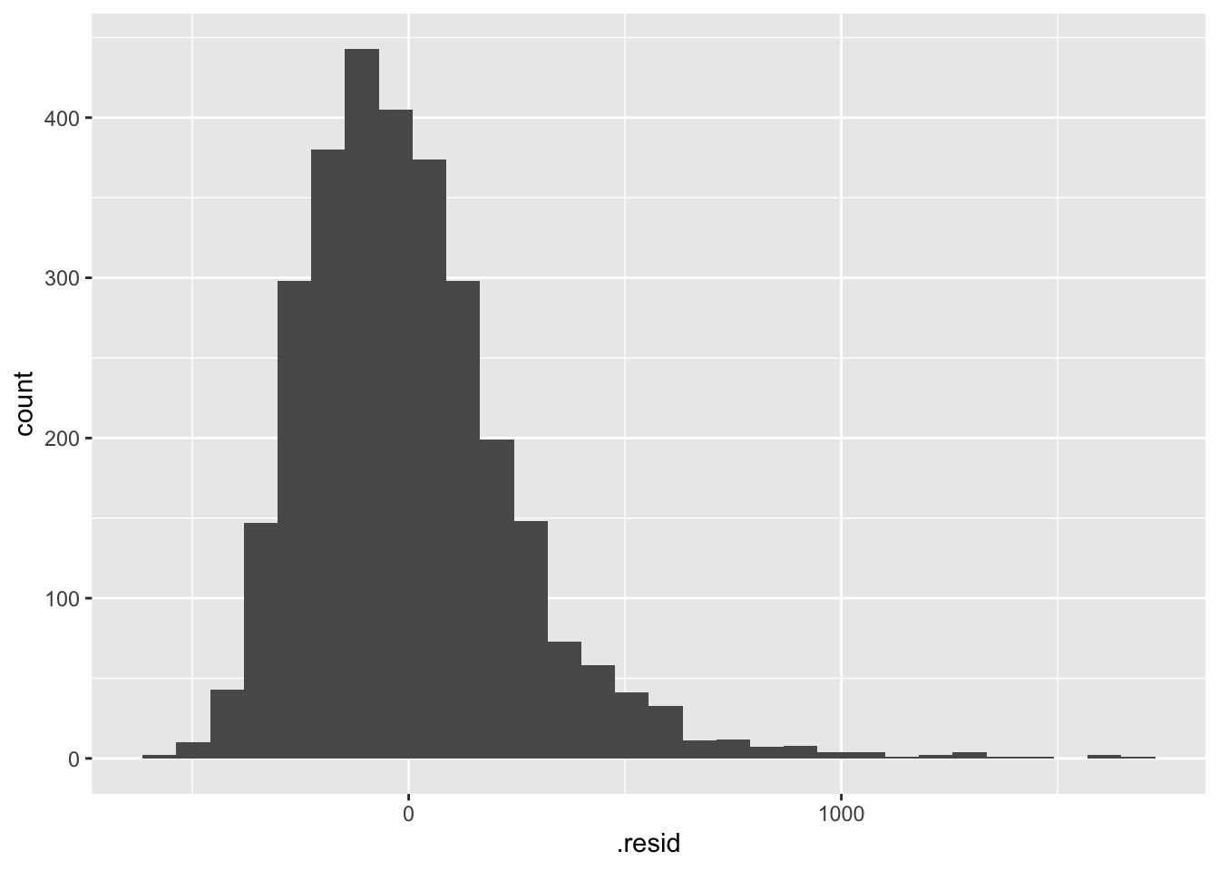

6 一連の操作をパイプでつなげる

broomの関数はパイプ演算子と相性が良いため，データの読み込みから推定結果の整理までを一気に記述できます．

read_csv("wage.csv", show_col_types = FALSE) %>%
  lm(wage ~ educ + exper, data = .) %>%
  tidy(conf.int = TRUE)

# A tibble: 3 × 7
  term        estimate std.error statistic   p.value conf.low conf.high
  <chr>          <dbl>     <dbl>     <dbl>     <dbl>    <dbl>     <dbl>
1 (Intercept)   -376.      37.8      -9.94 6.54e- 23   -450.     -301. 
2 educ            55.1      2.14     25.7  4.72e-132     50.9      59.3
3 exper           25.1      1.38     18.2  4.10e- 70     22.4      27.9

ここで，data = .の.は，パイプで渡されたオブジェクトを意味します．lm()関数の第1引数はモデル式であり，データフレームではないため，明示的にdata = .と指定する必要があります．

1 broomとは

2 準備：回帰分析の実行

3 tidy()：係数の整理

4 glance()：モデル全体の要約

5 augment()：予測値と残差の追加

6 一連の操作をパイプでつなげる

3 `tidy()`：係数の整理

4 `glance()`：モデル全体の要約

5 `augment()`：予測値と残差の追加