library(dplyr)
library(ggplot2)
library(patchwork)
library(broom)
library(fixest)
library(modelsummary)第13章のRコード
第13章 実証分析の手順
パッケージの読み込み
13.1 データを集める
13.1.2 Rの組み込みデータ
data()

help("datasets")

plot(women)

lm(height ~ weight,
   data = women)
13.1.6 データをながめる
malesdata <- readr::read_csv("Males1980.csv")

malesdata
# A tibble: 545 × 3
school exper wage
<dbl> <dbl> <dbl>
1 14 1 1.20
2 13 4 1.68
3 12 4 1.52
4 12 2 1.89
5 12 5 1.95
6 10 2 0.259
7 13 2 1.74
8 12 2 1.21
9 11 2 0.502
10 10 2 1.01
# ℹ 535 more rowsmalesdata %>%
summary() school exper wage
Min. : 3.00 Min. : 0.000 Min. :-1.114
1st Qu.:11.00 1st Qu.: 2.000 1st Qu.: 1.165
Median :12.00 Median : 3.000 Median : 1.448
Mean :11.77 Mean : 3.015 Mean : 1.393
3rd Qu.:12.00 3rd Qu.: 4.000 3rd Qu.: 1.742
Max. :16.00 Max. :11.000 Max. : 2.822 View(malesdata)g1 <- malesdata %>%
ggplot(aes(x = wage)) +
geom_histogram(bins = 15)
g2 <- malesdata %>%
ggplot(aes(x = school)) +
geom_histogram(bins = 15)
g3 <- malesdata %>%
ggplot(aes(x = exper)) +
geom_histogram(bins = 15)
g1 + g2 + g3 + plot_layout(ncol = 1)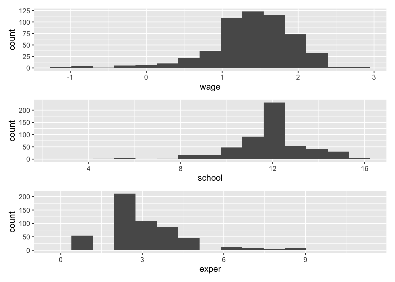
13.1.7 データの相関
cor(malesdata) school exper wage
school 1.0000000 -0.57975653 0.18114299
exper -0.5797565 1.00000000 0.07689126
wage 0.1811430 0.07689126 1.0000000013.2 推定結果を検証する
13.2.1 統計的有意性を確認する
malesdata %>%
  lm(wage ~ school + exper,
     data = .) %>%
  tidy()
# A tibble: 3 × 5
term estimate std.error statistic p.value
<chr> <dbl> <dbl> <dbl> <dbl>
1 (Intercept) -0.161 0.224 -0.718 4.73e- 1
2 school 0.108 0.0161 6.73 4.22e-11
3 exper 0.0923 0.0170 5.43 8.66e- 8malesdata %>%
lm(wage ~ school + exper,
data = .) %>%
glance() %>%
select(r.squared)# A tibble: 1 × 1
r.squared
<dbl>
1 0.082713.2.2 モデルを変えてみる
malesdata <- readr::read_csv("Males.csv")

malesdata <- malesdata %>%
  mutate(black      = 1 * (ethn == "black"),
         industry   = as.factor(industry),
         industry   = relevel(industry, ref = "Manufacturing"),
         occupation = as.factor(occupation),
         occupation = relevel(occupation, ref = "Clerical_and_kindred"))

malesdata %>%
  filter(year == 1980) %>%
  lm(wage ~ school + exper + black + health + married +
       union + industry + occupation,
     data = .) %>%
  tidy() %>%
  filter(p.value < 0.01)
# A tibble: 8 × 5
term estimate std.error statistic p.value
<chr> <dbl> <dbl> <dbl> <dbl>
1 school 0.0847 0.0166 5.11 4.43e-7
2 exper 0.0625 0.0170 3.67 2.69e-4
3 marriedyes 0.158 0.0596 2.66 8.08e-3
4 unionyes 0.210 0.0543 3.87 1.24e-4
5 industryEntertainment -0.698 0.204 -3.42 6.74e-4
6 industryMining -0.577 0.216 -2.68 7.66e-3
7 industryProfessional_and_Related Service -0.356 0.101 -3.53 4.44e-4
8 industryTrade -0.217 0.0708 -3.07 2.29e-3malesdata %>%
filter(year == 1980) %>%
lm(wage ~ school + exper + black + health + married +
union + industry + occupation,
data = .) %>%
glance() %>%
select(r.squared)# A tibble: 1 × 1
r.squared
<dbl>
1 0.21013.2.3 データを変えてみる
malesdata %>%
  feols(wage ~ school + exper + black + health + married +
       union + industry + occupation,
     data = .) %>%
  tidy() %>%
  filter(p.value < 0.01)
# A tibble: 15 × 5
term estimate std.error statistic p.value
<chr> <dbl> <dbl> <dbl> <dbl>
1 (Intercept) 0.418 0.0695 6.02 1.93e- 9
2 school 0.0845 0.00471 17.9 2.31e-69
3 exper 0.0434 0.00281 15.5 1.37e-52
4 black -0.127 0.0224 -5.66 1.65e- 8
5 marriedyes 0.0838 0.0152 5.52 3.55e- 8
6 unionyes 0.182 0.0172 10.6 6.40e-26
7 industryAgricultural -0.378 0.0524 -7.22 6.01e-13
8 industryBusiness_and_Repair_Service -0.143 0.0294 -4.87 1.13e- 6
9 industryConstruction -0.0898 0.0297 -3.02 2.51e- 3
10 industryEntertainment -0.522 0.0597 -8.74 3.23e-18
11 industryPersonal_Service -0.150 0.0571 -2.63 8.57e- 3
12 industryProfessional_and_Related Servi… -0.319 0.0312 -10.2 3.50e-24
13 industryTrade -0.225 0.0210 -10.8 1.16e-26
14 occupationManagers, Officials_and_Prop… 0.136 0.0318 4.28 1.94e- 5
15 occupationProfessional, Technical_and_… 0.158 0.0317 4.97 6.95e- 713.2.4 推定手法を変えてみる
malesdata %>%
  feols(wage ~ school + exper + black + health + married +
          union + industry + occupation | nr + year) %>%
  tidy() %>%
  filter(p.value < 0.01)
The variables 'school', 'exper' and 'black' have been removed because of collinearity (see $collin.var).# A tibble: 4 × 5
term estimate std.error statistic p.value
<chr> <dbl> <dbl> <dbl> <dbl>
1 unionyes 0.0828 0.0221 3.75 1.95e-4
2 industryEntertainment -0.223 0.0685 -3.25 1.23e-3
3 industryTrade -0.106 0.0274 -3.87 1.23e-4
4 occupationManagers, Officials_and_Propri… 0.0896 0.0320 2.79 5.38e-3補足:テーブルの作成方法
記述統計表
malesdata <- readr::read_csv("Males.csv")

malesdata %>%
datasummary_skim(histogram = FALSE)| Unique (#) | Missing (%) | Mean | SD | Min | Median | Max | |
|---|---|---|---|---|---|---|---|
| ...1 | 4360 | 0 | 2180.5 | 1258.8 | 1.0 | 2180.5 | 4360.0 |
| nr | 545 | 0 | 5262.1 | 3496.1 | 13.0 | 4569.0 | 12548.0 |
| year | 8 | 0 | 1983.5 | 2.3 | 1980.0 | 1983.5 | 1987.0 |
| school | 13 | 0 | 11.8 | 1.7 | 3.0 | 12.0 | 16.0 |
| exper | 19 | 0 | 6.5 | 2.8 | 0.0 | 6.0 | 18.0 |
| wage | 3631 | 0 | 1.6 | 0.5 | −3.6 | 1.7 | 4.1 |
malesdata <- malesdata %>%
  mutate(union   = 1 * (union   == "yes"),
         black   = 1 * (ethn    == "black"),
         married = 1 * (married == "yes"),
         health  = 1 * (health  == "yes"))

malesdata %>%
  select(wage, married, union, health,
         school, exper, black) %>%
  datasummary_skim(histogram = FALSE,
fmt = "%.2f")| Unique (#) | Missing (%) | Mean | SD | Min | Median | Max | |
|---|---|---|---|---|---|---|---|
| wage | 3631 | 0 | 1.65 | 0.53 | −3.58 | 1.67 | 4.05 |
| married | 2 | 0 | 0.44 | 0.50 | 0.00 | 0.00 | 1.00 |
| union | 2 | 0 | 0.24 | 0.43 | 0.00 | 0.00 | 1.00 |
| health | 2 | 0 | 0.02 | 0.13 | 0.00 | 0.00 | 1.00 |
| school | 13 | 0 | 11.77 | 1.75 | 3.00 | 12.00 | 16.00 |
| exper | 19 | 0 | 6.51 | 2.83 | 0.00 | 6.00 | 18.00 |
| black | 2 | 0 | 0.12 | 0.32 | 0.00 | 0.00 | 1.00 |
推定結果表
m1 <- malesdata %>%
  feols(wage ~ married + union + health +
          school + exper + black)

m2 <- malesdata %>%
  feols(wage ~ married + union + health +
          school + exper + black + industry + occupation)

m3 <- malesdata %>%
  feols(wage ~ married + union + health +
          school + exper + black + industry + occupation | nr + year)
The variables 'school', 'exper' and 'black' have been removed because of collinearity (see $collin.var).list(m1, m2, m3) %>%
modelsummary()| Model 1 | Model 2 | Model 3 | |
|---|---|---|---|
| (Intercept) | 0.034 | 0.040 | |
| (0.062) | (0.084) | ||
| married | 0.112 | 0.084 | 0.051 |
| (0.016) | (0.015) | (0.021) | |
| union | 0.184 | 0.182 | 0.083 |
| (0.017) | (0.017) | (0.022) | |
| health | −0.052 | −0.033 | −0.009 |
| (0.057) | (0.054) | (0.048) | |
| school | 0.103 | 0.084 | |
| (0.004) | (0.005) | ||
| exper | 0.050 | 0.043 | |
| (0.003) | (0.003) | ||
| black | −0.145 | −0.127 | |
| (0.023) | (0.022) | ||
| industryBusiness_and_Repair_Service | 0.235 | 0.016 | |
| (0.057) | (0.072) | ||
| industryConstruction | 0.288 | −0.005 | |
| (0.057) | (0.079) | ||
| industryEntertainment | −0.143 | −0.148 | |
| (0.077) | (0.088) | ||
| industryFinance | 0.410 | 0.204 | |
| (0.064) | (0.087) | ||
| industryManufacturing | 0.378 | 0.074 | |
| (0.052) | (0.065) | ||
| industryMining | 0.479 | 0.043 | |
| (0.075) | (0.113) | ||
| industryPersonal_Service | 0.228 | 0.064 | |
| (0.075) | (0.082) | ||
| industryProfessional_and_Related Service | 0.060 | −0.015 | |
| (0.058) | (0.076) | ||
| industryPublic_Administration | 0.292 | 0.056 | |
| (0.062) | (0.076) | ||
| industryTrade | 0.153 | −0.032 | |
| (0.053) | (0.065) | ||
| industryTransportation | 0.411 | 0.045 | |
| (0.058) | (0.070) | ||
| occupationCraftsmen, Foremen_and_kindred | 0.031 | 0.046 | |
| (0.028) | (0.031) | ||
| occupationFarm_Laborers_and_Foreman | −0.059 | 0.055 | |
| (0.078) | (0.074) | ||
| occupationLaborers_and_farmers | −0.067 | 0.040 | |
| (0.032) | (0.032) | ||
| occupationManagers, Officials_and_Proprietors | 0.136 | 0.090 | |
| (0.032) | (0.032) | ||
| occupationOperatives_and_kindred | −0.059 | 0.039 | |
| (0.028) | (0.027) | ||
| occupationProfessional, Technical_and_kindred | 0.158 | 0.092 | |
| (0.032) | (0.036) | ||
| occupationSales_Workers | 0.079 | 0.027 | |
| (0.037) | (0.053) | ||
| occupationService_Workers | −0.077 | 0.043 | |
| (0.030) | (0.039) | ||
| Num.Obs. | 4360 | 4360 | 4360 |
| R2 | 0.184 | 0.261 | 0.622 |
| R2 Adj. | 0.183 | 0.257 | 0.565 |
| R2 Within | 0.024 | ||
| R2 Within Adj. | 0.018 | ||
| AIC | 6010.2 | 5615.2 | 2684.9 |
| BIC | 6061.2 | 5787.5 | 2831.6 |
| RMSE | 0.48 | 0.46 | 0.33 |
| Std.Errors | IID | IID | by: nr |
| FE: nr | X | ||
| FE: year | X |
rows <- tribble(~term, ~`Model 1`, ~`Model 2`, ~`Model 3`,
                "Industry",      "No", "Yes", "Yes",
                "Occupation",    "No", "Yes", "Yes",
                "Individual FE", "No", "No",  "Yes",
                "Year FE",       "No", "No",  "Yes")

attr(rows, "position") <- 15:18

msummary(list(m1, m2, m3),
         coef_omit   = "industry|occupation",
         coef_rename = c("(Intercept)" = "切片"),
         gof_map     = "nobs",
         add_rows    = rows,
         stars       = TRUE,
notes = "備考:対数賃金を被説明変数として線形回帰モデルを最小二乗法により推定して得られた推定値。丸括弧内は標準誤差。")| Model 1 | Model 2 | Model 3 | |||||
|---|---|---|---|---|---|---|---|
| 切片 | 0.034 | 0.040 | |||||
| (0.062) | (0.084) | ||||||
| married | 0.112*** | 0.084*** | 0.051* | ||||
| (0.016) | (0.015) | (0.021) | |||||
| union | 0.184*** | 0.182*** | 0.083*** | ||||
| (0.017) | (0.017) | (0.022) | |||||
| health | −0.052 | −0.033 | −0.009 | ||||
| (0.057) | (0.054) | (0.048) | |||||
| school | 0.103*** | 0.084*** | |||||
| (0.004) | (0.005) | ||||||
| exper | 0.050*** | 0.043*** | |||||
| (0.003) | (0.003) | ||||||
| black | −0.145*** | −0.127*** | |||||
| (0.023) | (0.022) | ||||||
| Industry | No | Yes | Yes | ||||
| Occupation | No | Yes | Yes | ||||
| Individual FE | No | No | Yes | ||||
| Year FE | No | No | Yes | ||||
| Num.Obs. | 4360 | 4360 | 4360 | ||||
| + p < 0.1, * p < 0.05, ** p < 0.01, *** p < 0.001 | |||||||
| 備考:対数賃金を被説明変数として線形回帰 モデルを最小二乗法により推定して得られた 推定値。丸括弧内は標準誤差。 |