library(dplyr)
library(ggplot2)
library(rdd)
library(broom)
library(purrr)
library(tidyr)第10章のRコード
第10章 不連続回帰デザイン
パッケージの読み込み
10.2 条件付平均トリートメント効果 \(\tau\) の推定
10.2.1 条件付期待値が線形の場合
examdata <- readr::read_csv("exam_rdd.csv")

examdata %>%
  print(n = 4)
# A tibble: 200 × 2
Y Z
<dbl> <dbl>
1 72.7 57.0
2 76.9 75.3
3 51.0 64.3
4 77.2 73.3
# ℹ 196 more rowsexamdata <- examdata %>%
mutate(D = ifelse(Z < 60, 1, 0))
examdata %>%
mutate(Zc = Z - 60) %>%
lm(Y ~ D + Zc + D:Zc,
data = .) %>%
tidy()# A tibble: 4 × 5
term estimate std.error statistic p.value
<chr> <dbl> <dbl> <dbl> <dbl>
1 (Intercept) 60.1 1.46 41.3 1.34e-98
2 D 13.0 2.03 6.41 1.05e- 9
3 Zc 0.826 0.115 7.15 1.65e-11
4 D:Zc -0.165 0.167 -0.985 3.26e- 110.2.2 条件付期待値が非線形の場合
h <- 5
examdata %>%
  mutate(Zc = Z - 60) %>%
  filter(abs(Zc) <= h) %>% # Z - c が - h 未満または h を超えるものを除外
  lm(Y ~ D,
     data = .) %>%
  tidy()
# A tibble: 2 × 5
term estimate std.error statistic p.value
<chr> <dbl> <dbl> <dbl> <dbl>
1 (Intercept) 62.1 1.61 38.5 8.72e-50
2 D 10.7 2.11 5.04 3.34e- 6examdata %>%
mutate(Zc = Z - 60) %>%
filter(abs(Zc) <= h) %>% # Z - c が - h 未満または h を超えるものを除外
lm(Y ~ D * Zc,
data = .) %>%
tidy()# A tibble: 4 × 5
term estimate std.error statistic p.value
<chr> <dbl> <dbl> <dbl> <dbl>
1 (Intercept) 63.7 3.59 17.7 1.37e-27
2 D 10.3 4.69 2.20 3.15e- 2
3 Zc -0.609 1.21 -0.502 6.17e- 1
4 D:Zc 1.06 1.55 0.682 4.97e- 1Rによるデータ演習
electdata <- readr::read_csv("incumbency.csv")

electdata %>%
  print(n = 4)
# A tibble: 6,559 × 2
voteshare margin
<dbl> <dbl>
1 0.581 0.105
2 0.461 0.139
3 0.543 -0.0736
4 0.585 0.0868
# ℹ 6,555 more rowselectdata <- electdata %>%
mutate(D = 1 * (margin >= 0))electdata %>%
ggplot(aes(x = margin, y = voteshare)) +
geom_point() +
geom_vline(xintercept = 0,
linetype = "dashed") +
xlab("前回の得票率 - 当落線") +
ylab("得票率") +
theme_gray(base_family = "HiraKakuPro-W3")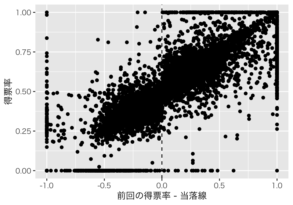
electdata %>%
  pull(margin) %>%
  DCdensity(cutpoint = 0,
            plot = FALSE)
[1] 0.1792064h <- 0.25
electdata %>%
lm(voteshare ~ D + margin + D:margin,
data = .,
subset = abs(margin) <= h) %>%
tidy()# A tibble: 4 × 5
term estimate std.error statistic p.value
<chr> <dbl> <dbl> <dbl> <dbl>
1 (Intercept) 0.451 0.00607 74.3 0
2 D 0.0817 0.00844 9.67 8.86e-22
3 margin 0.367 0.0432 8.48 3.56e-17
4 D:margin 0.0849 0.0607 1.40 1.62e- 1h <- 0.05
electdata %>%
lm(voteshare ~ D + margin + D:margin,
data = .,
subset = abs(margin) <= h) %>%
tidy()# A tibble: 4 × 5
term estimate std.error statistic p.value
<chr> <dbl> <dbl> <dbl> <dbl>
1 (Intercept) 0.469 0.0139 33.7 2.84e-141
2 D 0.0454 0.0189 2.40 1.66e- 2
3 margin 0.903 0.481 1.88 6.10e- 2
4 D:margin 0.110 0.645 0.171 8.65e- 1result <- tibble(h = seq(0.01, 0.25, 0.01))
results <- result %>%
group_by(h) %>%
mutate(
reg = map(h, ~ lm(voteshare ~ D * margin,
data = electdata,
subset = (abs(margin) <= h))),
tidied = map(reg, tidy, conf.int = TRUE)
) %>%
unnest(tidied) %>%
filter(term == "D") results %>%
ggplot(aes(x = h, y = estimate, ymin = conf.low, ymax = conf.high)) +
geom_point() +
geom_pointrange() +
geom_hline(yintercept = 0, linetype = "dashed") +
xlab("バンド幅") +
ylab("トリートメント効果の推定値") +
theme_gray(base_family = "HiraKakuPro-W3")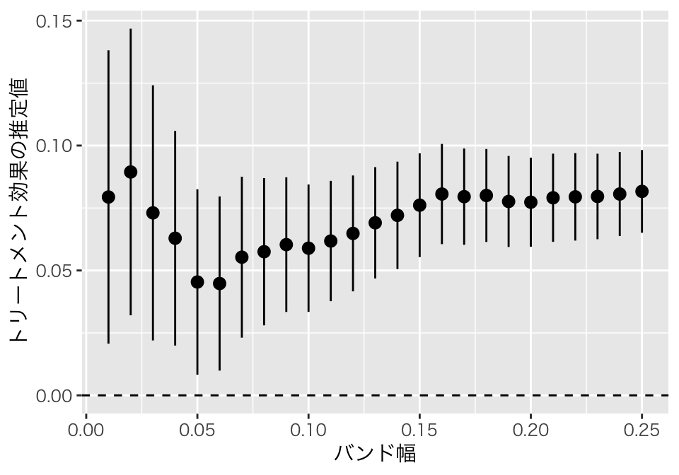
result_ik <- RDestimate(voteshare ~ margin,
                        data = electdata,
                        cutpoint = 0,
                        kernel = "rectangular")

summary(result_ik)
Call:
RDestimate(formula = voteshare ~ margin, data = electdata, cutpoint = 0,
    kernel = "rectangular")

Type:
sharp

Estimates:
           Bandwidth  Observations  Estimate  Std. Error  z value  Pr(>|z|)
LATE       0.3768     3986          0.08837   0.007018    12.592   2.335e-36
Half-BW    0.1884     2156          0.07934   0.009435     8.409   4.150e-17
Double-BW  0.7535     5654          0.06903   0.005764    11.976   4.759e-33

LATE       ***
Half-BW    ***
Double-BW  ***
---
Signif. codes:  0 '***' 0.001 '**' 0.01 '*' 0.05 '.' 0.1 ' ' 1

F-statistics:
           F       Num. DoF  Denom. DoF  p
LATE       1242.0  3         3982        0
Half-BW     396.4  3         2152        0
Double-BW  3296.0  3         5650        0