library(dplyr)
library(tidyr)
library(ggplot2)第1章のRコード
第1章 回帰分析の目的
パッケージの呼び出し
図 1.1 (体重と身長)
women %>%
  ggplot(aes(x = weight,
             y = height)) +
  geom_point()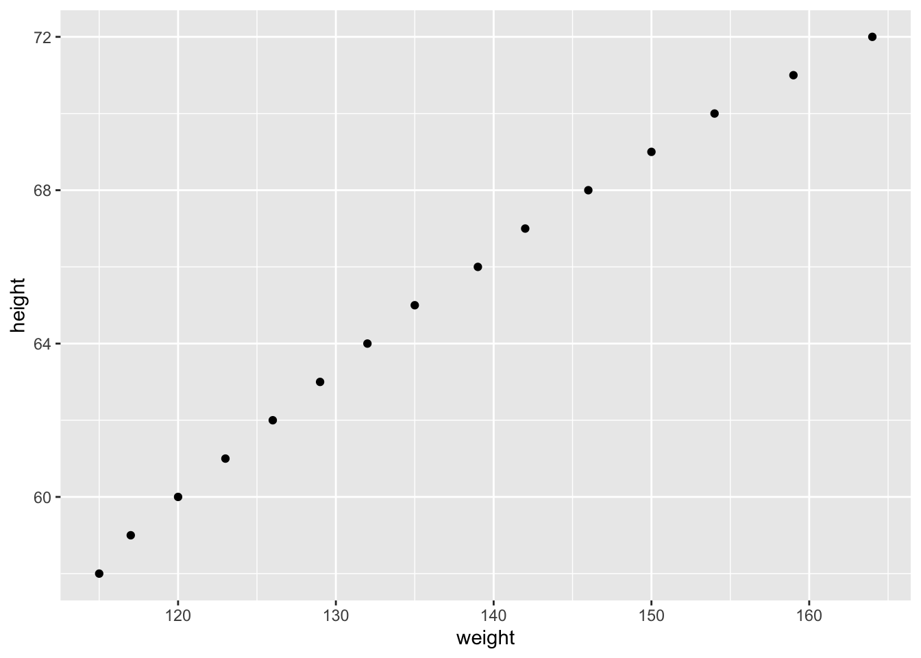
図 1.2 (タバコと健康)
USPersonalExpenditure %>%
  as_tibble(rownames = "item") %>%
  pivot_longer(`1940`:`1960`,
               names_to  = "year",
               values_to = "expenditure") %>%
  pivot_wider(names_from  = item,
              values_from = expenditure) %>%
  ggplot(aes(x = `Food and Tobacco`,
             y = `Medical and Health`)) +
  geom_point() +
  geom_line() +
  xlab("食料品およびタバコへの支出額") +
  ylab("医療および健康への支出総額") +
  theme_gray(base_family = "HiraKakuPro-W3")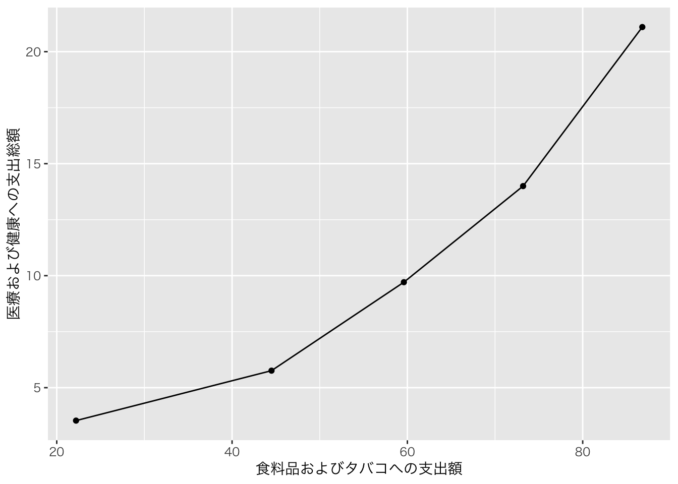
表 1.1 (アメリカにおける個人支出額)
USPersonalExpenditure %>%
  kableExtra::kbl() %>%
kableExtra::kable_classic_2()| 1940 | 1945 | 1950 | 1955 | 1960 | |
|---|---|---|---|---|---|
| Food and Tobacco | 22.200 | 44.500 | 59.60 | 73.2 | 86.80 |
| Household Operation | 10.500 | 15.500 | 29.00 | 36.5 | 46.20 |
| Medical and Health | 3.530 | 5.760 | 9.71 | 14.0 | 21.10 |
| Personal Care | 1.040 | 1.980 | 2.45 | 3.4 | 5.40 |
| Private Education | 0.341 | 0.974 | 1.80 | 2.6 | 3.64 |
USPersonalExpenditure %>%
  kableExtra::kbl(format = "latex", booktabs = TRUE) %>%
kableExtra::kable_classic_2()\begin{table}
\centering
\begin{tabular}[t]{lrrrrr}
\toprule
& 1940 & 1945 & 1950 & 1955 & 1960\\
\midrule
Food and Tobacco & 22.200 & 44.500 & 59.60 & 73.2 & 86.80\\
Household Operation & 10.500 & 15.500 & 29.00 & 36.5 & 46.20\\
Medical and Health & 3.530 & 5.760 & 9.71 & 14.0 & 21.10\\
Personal Care & 1.040 & 1.980 & 2.45 & 3.4 & 5.40\\
Private Education & 0.341 & 0.974 & 1.80 & 2.6 & 3.64\\
\bottomrule
\end{tabular}
\end{table}図 1.3 (各種支出額の相関)
usp <- USPersonalExpenditure %>%
  as_tibble(rownames = "item") %>%
  pivot_longer(`1940`:`1960`,
               names_to  = "year",
               values_to = "expenditure") %>%
  pivot_wider(names_from  = item,
              values_from = expenditure)
g1 <- usp %>%
ggplot(aes(x = `Food and Tobacco`,
y = `Household Operation`)) +
geom_point() +
geom_line()
g2 <- usp %>%
ggplot(aes(x = `Medical and Health`,
y = `Household Operation`)) +
geom_point() +
geom_line()
g3 <- usp %>%
ggplot(aes(x = `Private Education`,
y = `Household Operation`)) +
geom_point() +
geom_line()
g4 <- usp %>%
ggplot(aes(x = `Food and Tobacco`,
y = `Personal Care`)) +
geom_point() +
geom_line()
g5 <- usp %>%
ggplot(aes(x = `Medical and Health`,
y = `Personal Care`)) +
geom_point() +
geom_line()
g6 <- usp %>%
ggplot(aes(x = `Private Education`,
y = `Personal Care`)) +
geom_point() +
geom_line()library(patchwork)
g1 + g2 + g3 +
g4 + g5 + g6 +
plot_layout(ncol = 3)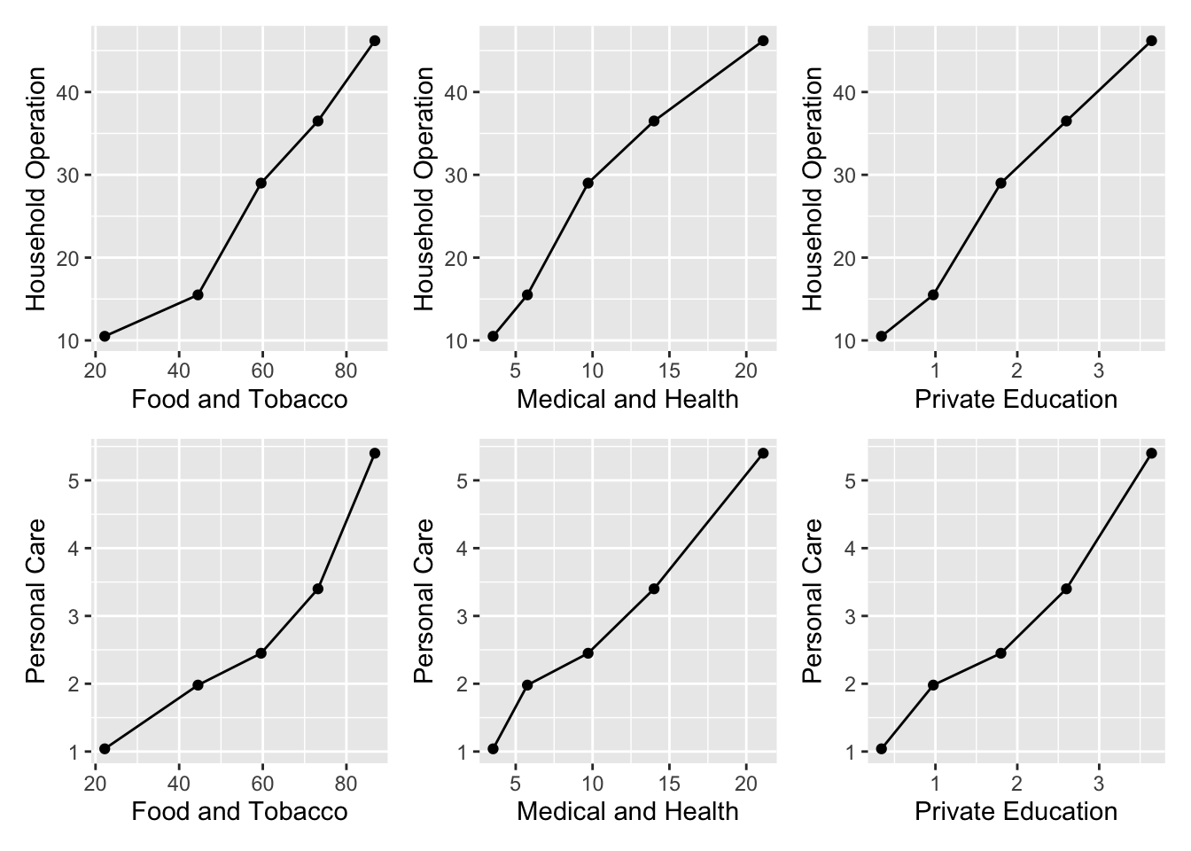
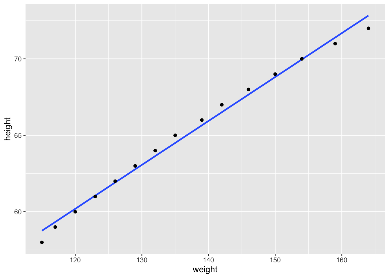
図 1.5 (身長の体重への回帰直線)
women %>%
  ggplot(aes(x = weight,
             y = height)) +
  geom_smooth(method = "lm", se = FALSE) +
  geom_point()