library(dplyr)
library(lubridate)
library(broom)第5章のRコード
第5章 推測統計の基礎
パッケージの読み込み
5.1 統計的仮説検定の考え方
5.1.3 コイン投げの例
p40 <- pbinom(q = 40, size = 100, prob = 0.5)
p60 <- pbinom(q = 60, size = 100, prob = 0.5)
p60 - p40
[1] 0.95395595.2 平均値の検定
5.2.5 Rによる例題演習
simdata <- readr::read_csv("distributions.csv")

simdata %>%
  summarise(mean_A = mean(distA),
            var_A  = var(distA))
# A tibble: 1 × 2
mean_A var_A
<dbl> <dbl>
1 2.04 0.373simdata %>%
summarise(mean_A = mean(distA),
var_A = var(distA),
t.value = sqrt(100) / sqrt(var_A) * mean_A)# A tibble: 1 × 3
mean_A var_A t.value
<dbl> <dbl> <dbl>
1 2.04 0.373 33.45.2.6 \(p\)値
1 - pnorm(1.250113) + pnorm(-1.250113)[1] 0.21125835.3 回帰係数の検定
5.3.2 \(\hat{\beta}_1\)の分布のシミュレーション
set.seed(2022)

X <- rnorm(1000, 0, 1)
Y <- 1 + 5 * X + rnorm(1000, 0, 1)

beta1 <- lm(Y ~ X)$coefficients

names(lm(Y ~ X))
[1] "coefficients" "residuals" "effects" "rank"
[5] "fitted.values" "assign" "qr" "df.residual"
[9] "xlevels" "call" "terms" "model" S <- 10000
beta1 <- numeric(S) # 結果の保存
for(i in 1:S){ # 繰り返し開始
x <- rnorm(1000, 0, 1)
y <- 1 + 5 * x + rnorm(1000, 0, 1)
beta1[i] <- lm(y ~ x)$coefficients[2]
} # 繰り返し終了summary(beta1) # 結果の要約 Min. 1st Qu. Median Mean 3rd Qu. Max.
4.885 4.979 5.000 5.000 5.022 5.115 sd(beta1) # 標準偏差[1] 0.03176331hist(beta1) # 結果の描画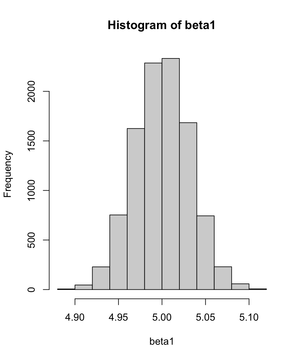
5.3.6 Rによる分析例
wagedata <- readr::read_csv("wage.csv")

wagedata %>%
  lm(log(wage) ~ educ + exper,
     data = .) %>%
  summary()
Call:
lm(formula = log(wage) ~ educ + exper, data = .)

Residuals:
     Min       1Q   Median       3Q      Max
-1.93442 -0.26396  0.02404  0.27287  1.42863

Coefficients:
            Estimate Std. Error t value Pr(>|t|)
(Intercept) 4.666034   0.063790   73.15   <2e-16 ***
educ        0.093168   0.003612   25.80   <2e-16 ***
exper       0.040657   0.002334   17.42   <2e-16 ***
---
Signif. codes:  0 '***' 0.001 '**' 0.01 '*' 0.05 '.' 0.1 ' ' 1

Residual standard error: 0.4017 on 3007 degrees of freedom
Multiple R-squared:  0.1813,    Adjusted R-squared:  0.1808
F-statistic:   333 on 2 and 3007 DF,  p-value: < 2.2e-16
0.093168 / 0.003612[1] 25.794025.4 信頼区間
5.4.2 Rによる分析例
result <- wagedata %>%
  lm(log(wage) ~ educ + exper,
     data = .)

summary(result)$coefficients
Estimate Std. Error t value Pr(>|t|)
(Intercept) 4.66603445 0.063790003 73.14680 0.000000e+00
educ 0.09316802 0.003611751 25.79581 1.000493e-132
exper 0.04065736 0.002334406 17.41658 8.434838e-65summary(result)$coefficients[, 1:2] Estimate Std. Error
(Intercept) 4.66603445 0.063790003
educ 0.09316802 0.003611751
exper 0.04065736 0.002334406betahat <- summary(result)$coefficients[, 1]
sigma <- summary(result)$coefficients[, 2]
lower <- betahat - 1.96 * sigma
upper <- betahat + 1.96 * sigma
cbind(lower, upper) lower upper
(Intercept) 4.54100604 4.7910629
educ 0.08608899 0.1002471
exper 0.03608193 0.0452328result %>% confint() 2.5 % 97.5 %
(Intercept) 4.54095799 4.79111090
educ 0.08608627 0.10024978
exper 0.03608017 0.04523456result %>% confint(level = 0.99) 0.5 % 99.5 %
(Intercept) 4.50161793 4.83045097
educ 0.08385886 0.10247719
exper 0.03464052 0.04667421補足
tempdata <- readr::read_csv("temperature_aug.csv")

tempdata <- tempdata %>% # 変数の作成・加工
  mutate(daytime = 1 * (18 >= time & time >= 9),
         date    = ymd(date),
         dow     = wday(date, label = TRUE),
         sunday  = 1 * (dow == "日"),
         recess  = 1 * ("2014-08-16" >= date & date >= "2014-08-11"))

result <- tempdata %>%
  lm(elec ~ temp + daytime + prec + sunday + recess,
     data = .)

result %>% tidy()
# A tibble: 6 × 5
term estimate std.error statistic p.value
<chr> <dbl> <dbl> <dbl> <dbl>
1 (Intercept) -0.332 123. -0.00269 9.98e- 1
2 temp 117. 4.55 25.7 2.09e-104
3 daytime 556. 32.4 17.2 6.56e- 56
4 prec -2.67 15.9 -0.168 8.67e- 1
5 sunday NA NA NA NA
6 recess -348. 37.4 -9.31 1.40e- 19result %>% glance()# A tibble: 1 × 12
r.squared adj.r.squared sigma statistic p.value df logLik AIC BIC
<dbl> <dbl> <dbl> <dbl> <dbl> <dbl> <dbl> <dbl> <dbl>
1 0.683 0.681 403. 398. 9.81e-183 4 -5517. 11046. 11073.
# ℹ 3 more variables: deviance <dbl>, df.residual <int>, nobs <int>result %>% augment()# A tibble: 744 × 12
elec temp daytime prec sunday recess .fitted .resid .hat .sigma
<dbl> <dbl> <dbl> <dbl> <dbl> <dbl> <dbl> <dbl> <dbl> <dbl>
1 3193 27.9 0 0 0 0 3262. -68.8 0.00284 403.
2 2960 27.9 0 0 0 0 3262. -302. 0.00284 403.
3 2807 27.1 0 0 0 0 3168. -361. 0.00267 403.
4 2748 26.8 0 0 0 0 3133. -385. 0.00265 403.
5 2735 26.9 0 0 0 0 3145. -410. 0.00265 403.
6 2736 27.3 0 0 0 0 3192. -456. 0.00270 403.
7 2950 28.3 0 0 0 0 3309. -359. 0.00299 403.
8 3336 29.4 0 0 0 0 3437. -101. 0.00361 403.
9 3863 30.2 0 0 0 0 3531. 332. 0.00425 403.
10 4328 32.2 1 0 0 0 4320. 7.65 0.00467 403.
# ℹ 734 more rows
# ℹ 2 more variables: .cooksd <dbl>, .std.resid <dbl>