第9章のRコード

第9章 マッチング法

サンプルデータ

wage_training.csv:研修と賃金に関する架空データ.

パッケージの読み込み

library(dplyr)
library(MatchIt)
library(broom)

Rによるデータ演習

wagedata <- readr::read_csv("wage_training.csv")
wagedata %>% 
  print(n = 4)
# A tibble: 800 × 6
  wagea     D years wageb  educ female
  <dbl> <dbl> <dbl> <dbl> <dbl>  <dbl>
1    19     1     4    18    17      1
2    27     0    22    27    13      0
3    20     1     2    18    15      1
4    36     1    14    34    14      1
# ℹ 796 more rows
wagedata %>% # トリートメントグループとコントロールグループの平均値の差
  summarise(mean_treated    = mean(wagea[D == 1]),
            mean_controlled = mean(wagea[D == 0]),
            mean_diff       = mean_treated - mean_controlled)
# A tibble: 1 × 3
  mean_treated mean_controlled mean_diff
         <dbl>           <dbl>     <dbl>
1         25.7            26.8     -1.13
wagedata %>% # 相関係数
  summarise(cor_years = cor(D, years),
            cor_wageb = cor(D, wageb))
# A tibble: 1 × 2
  cor_years cor_wageb
      <dbl>     <dbl>
1    -0.191    -0.184
m.out <- matchit(D ~ years + wageb,
                 data     = wagedata,
                 method   = "nearest",
                 distance = "scaled_euclidean",
                 replace  = TRUE)
m.out
A matchit object
 - method: 1:1 nearest neighbor matching with replacement
 - distance: Scaled Euclidean
 - number of obs.: 800 (original), 361 (matched)
 - target estimand: ATT
 - covariates: years, wageb
m.out %>% summary()

Call:
matchit(formula = D ~ years + wageb, data = wagedata, method = "nearest", 
    distance = "scaled_euclidean", replace = TRUE)

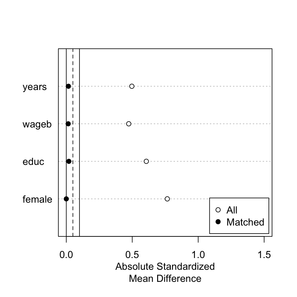
Summary of Balance for All Data:
      Means Treated Means Control Std. Mean Diff. Var. Ratio eCDF Mean eCDF Max
years        8.2311       10.9377         -0.4970     0.6556    0.1044   0.1722
wageb       24.4874       26.6637         -0.4734     0.6734    0.0989   0.2094


Summary of Balance for Matched Data:
      Means Treated Means Control Std. Mean Diff. Var. Ratio eCDF Mean eCDF Max
years        8.2311        8.2269          0.0008     1.0049    0.0047   0.0210
wageb       24.4874       24.4874          0.0000     0.9924    0.0008   0.0084
      Std. Pair Dist.
years          0.0239
wageb          0.0168

Sample Sizes:
              Control Treated
All            562.       238
Matched (ESS)   87.68     238
Matched        123.       238
Unmatched      439.         0
Discarded        0.         0
m.out_full <- matchit(D ~ years + wageb + educ + female,
                      data     = wagedata,
                      method   = "nearest",
                      distance = "scaled_euclidean",
                      replace  = TRUE)
m.out_full %>%
  summary() %>%
  plot(xlim = c(0, 1.5))

match.data(m.out)
# A tibble: 361 × 7
   wagea     D years wageb  educ female weights
   <dbl> <dbl> <dbl> <dbl> <dbl>  <dbl>   <dbl>
 1    19     1     4    18    17      1   1    
 2    27     0    22    27    13      0   1.03 
 3    20     1     2    18    15      1   1    
 4    36     1    14    34    14      1   1    
 5    18     0     4    18    11      1   2.58 
 6    29     0    19    29    15      0   1.03 
 7    21     1     3    20    18      1   1    
 8    31     0    13    31    15      1   1.03 
 9    26     0    13    26    14      0   3.10 
10    35     0    19    34    15      1   0.517
# ℹ 351 more rows
match.data(m.out) %>% 
  lm(wagea ~ D,
     data = .,
     weights = weights) %>% 
  tidy()
# A tibble: 2 × 5
  term        estimate std.error statistic   p.value
  <chr>          <dbl>     <dbl>     <dbl>     <dbl>
1 (Intercept)    24.6      0.413     59.7  2.11e-188
2 D               1.09     0.508      2.15 3.23e-  2
m.out <- matchit(D ~ years + wageb,
                 data     = wagedata,
                 method   = "nearest",
                 distance = "glm",
                 replace  = TRUE)

m.out %>% 
  match.data() %>% 
  lm(wagea ~ D,
       data = .,
     weights = weights) %>% 
  tidy()
# A tibble: 2 × 5
  term        estimate std.error statistic   p.value
  <chr>          <dbl>     <dbl>     <dbl>     <dbl>
1 (Intercept)   25.1       0.429     58.4  3.39e-184
2 D              0.639     0.526      1.21 2.25e-  1