第4章のPythonコード

4章回帰分析の基礎

サンプルデータ

temperature_aug.csv：2014年8月の東京都の気温データ．

wage.csv：1976年米国における男性労働者の賃金に関するデータ．

モジュールのインポート

import pandas as pd
import seaborn as sns
import matplotlib.pyplot as plt
import japanize_matplotlib
from statsmodels.formula.api import ols
import numpy as np
import datetime

4.1 回帰分析の考え方

4.1.4 数値例：気温と電力使用量

import plotly.io as pio
pio.renderers.default = 'notebook'

tempdata = pd.read_csv('temperature_aug.csv')

sns.set_theme(font='IPAexGothic')

fig = sns.relplot(x = 'time', y = 'temp', data = tempdata)

plt.xlabel("時刻")
plt.ylabel("気温")
plt.show()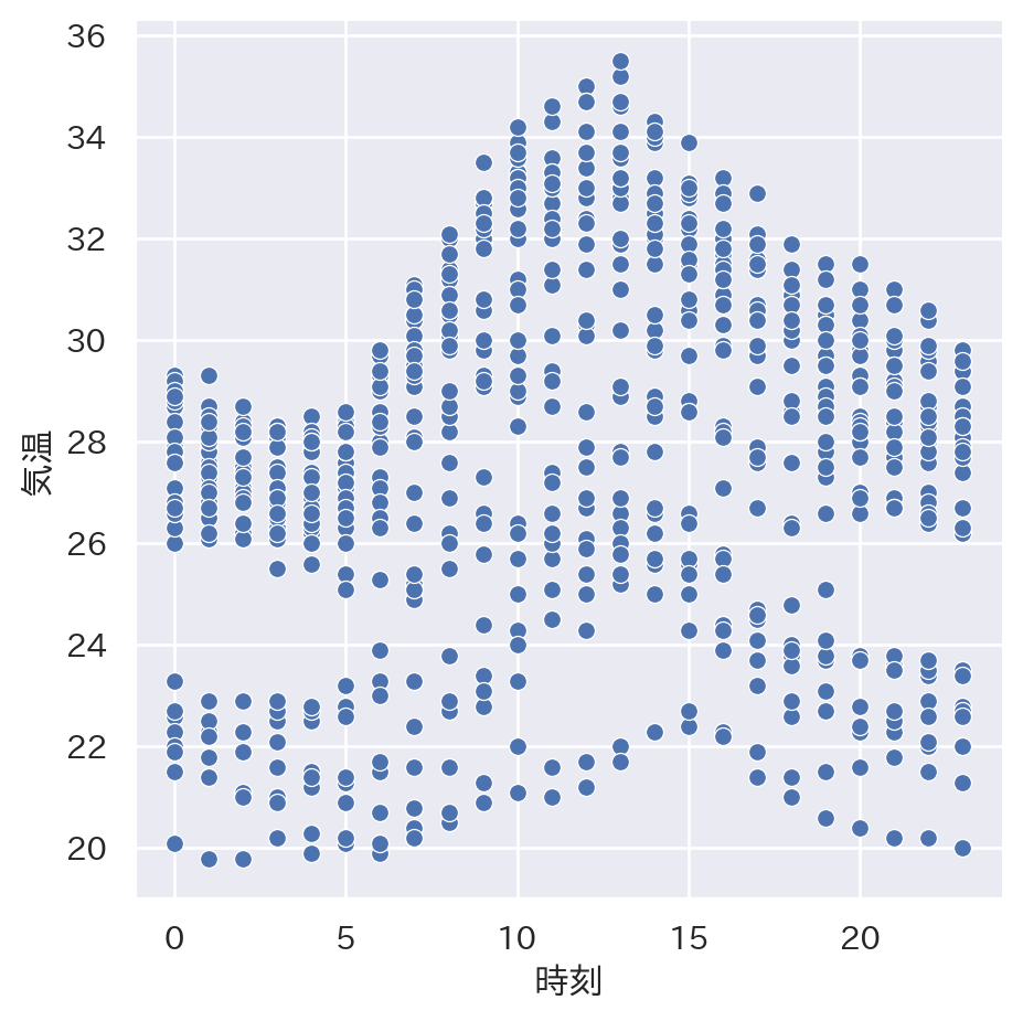

4.1.6 ノンパラメトリック回帰の実行

tempdata.describe()

	time	elec	prec	temp
count	744.000000	744.000000	744.000000	744.000000
mean	11.500000	3398.486559	0.141129	27.668414
std	6.926843	714.344671	0.945117	3.545453
min	0.000000	2213.000000	0.000000	19.800000
25%	5.750000	2823.500000	0.000000	25.675000
50%	11.500000	3342.500000	0.000000	28.000000
75%	17.250000	3871.500000	0.000000	30.125000
max	23.000000	4980.000000	17.000000	35.500000

time_temp = tempdata.groupby('time').mean(numeric_only = True)
time_temp

	elec	prec	temp
time
0	2914.064516	0.032258	26.361290
1	2717.774194	0.290323	26.096774
2	2605.483871	0.483871	25.896774
3	2567.419355	0.145161	25.835484
4	2563.645161	0.225806	25.725806
5	2562.548387	0.080645	25.832258
6	2703.806452	0.064516	26.425806
7	2991.161290	0.048387	27.258065
8	3383.225806	0.000000	28.135484
9	3730.225806	0.000000	29.038710
10	3868.290323	0.000000	29.422581
11	3948.483871	0.241935	29.622581
12	3884.225806	0.225806	29.874194
13	3954.709677	0.129032	30.038710
14	3964.322581	0.145161	29.706452
15	3935.354839	0.161290	29.309677
16	3935.774194	0.096774	28.880645
17	3872.064516	0.032258	28.290323
18	3911.419355	0.806452	27.716129
19	3854.903226	0.016129	27.454839
20	3678.903226	0.016129	27.187097
21	3484.258065	0.048387	26.938710
22	3376.677419	0.032258	26.629032
23	3154.935484	0.064516	26.364516

sns.relplot(x = 'time', y = 'temp', kind = 'line', data = time_temp)
plt.xlabel("時刻")
plt.ylabel("気温")
plt.show()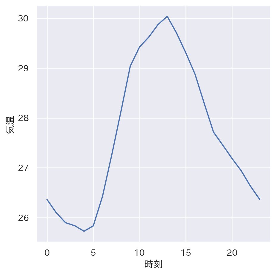

sns.lineplot(x = 'time', y = 'temp', errorbar = None, data = tempdata)
plt.xlabel("時刻")
plt.ylabel("気温")
plt.show()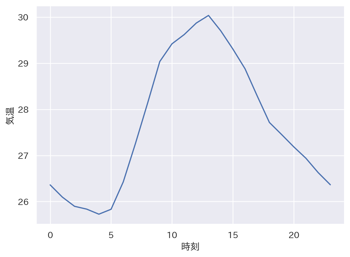

4.2 単回帰分析

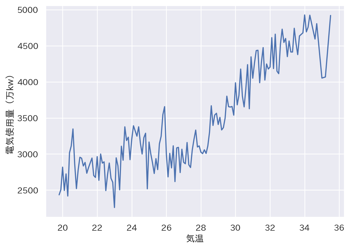
4.2.1 ノンパラメトリック回帰の限界

tempdata.corr()

/var/folders/xt/knmm4spn729b1ppxvlvvklc00000gn/T/ipykernel_24349/1573599017.py:1: FutureWarning:

The default value of numeric_only in DataFrame.corr is deprecated. In a future version, it will default to False. Select only valid columns or specify the value of numeric_only to silence this warning.

	time	elec	prec	temp
time	1.000000	0.499409	-0.020867	0.130154
elec	0.499409	1.000000	-0.080383	0.719818
prec	-0.020867	-0.080383	1.000000	-0.156318
temp	0.130154	0.719818	-0.156318	1.000000

sns.lineplot(x = 'temp', y = 'elec', ci = None, data = tempdata)
plt.xlabel("気温")
plt.ylabel("電気使用量（万kw）")
plt.show()

/var/folders/xt/knmm4spn729b1ppxvlvvklc00000gn/T/ipykernel_24349/1055470134.py:1: FutureWarning:



The `ci` parameter is deprecated. Use `errorbar=None` for the same effect.

4.2.4 Rによる線形回帰分析

result = ols('elec ~ temp', data = tempdata).fit()

result.params

Intercept   -614.272179
temp         145.030313
dtype: float64

sns.scatterplot(x = 'temp', y = 'elec', data = tempdata)
plt.axline(xy1 = (0, result.params[0]), slope = result.params[1])
plt.xlabel("気温")
plt.ylabel("電気使用量（万kw）")
plt.xlim([19, 36])
plt.ylim([2100, 5100])
plt.show()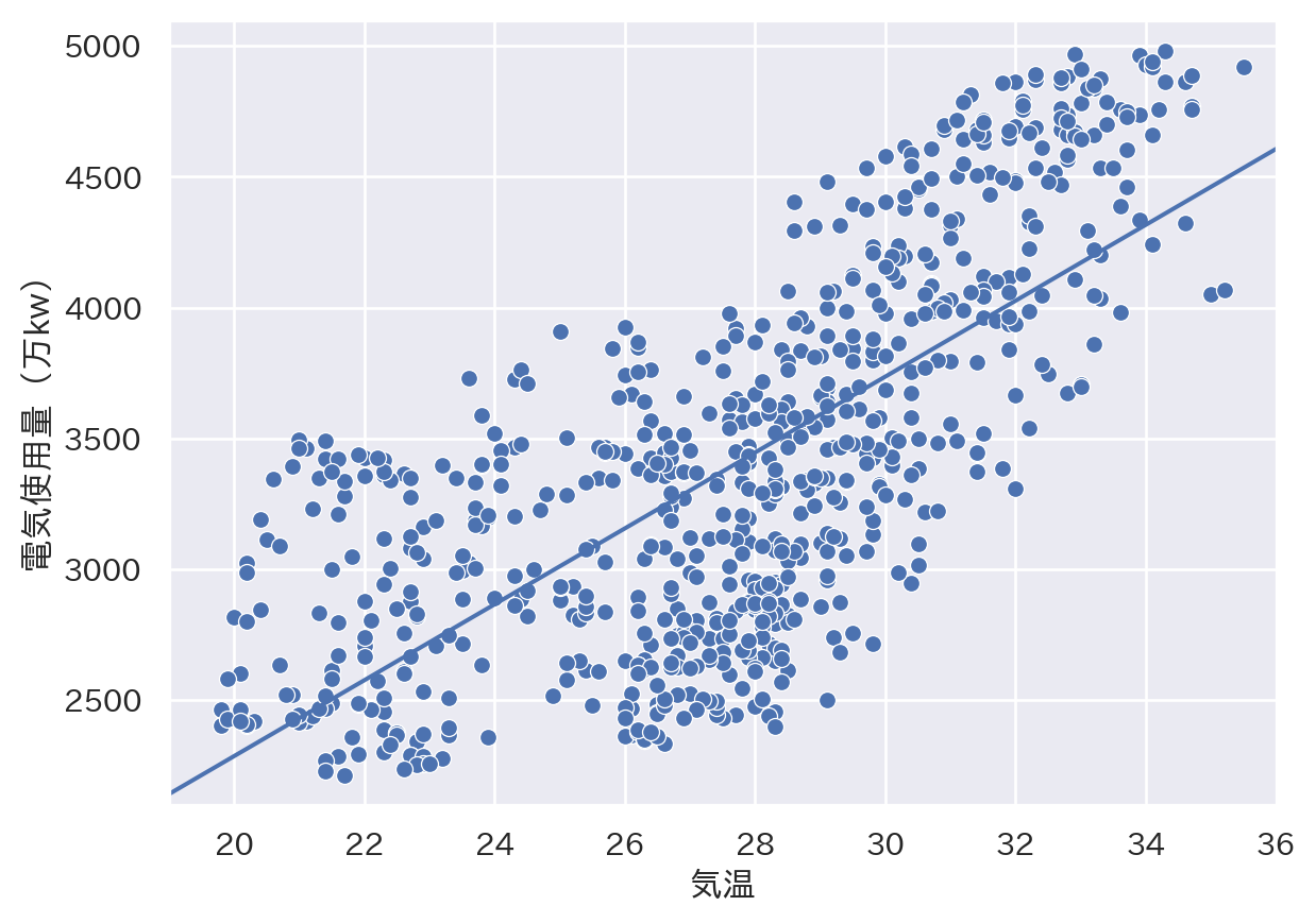

sns.regplot(x = 'temp', y = 'elec', ci = None, data = tempdata)
plt.xlabel("気温")
plt.ylabel("電気使用量（万kw）")
plt.show()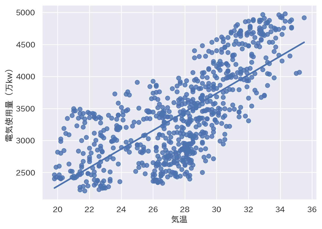

4.3 重回帰分析

4.3.1 説明変数を追加する

sns.scatterplot(x = 'time', y = 'elec', data = tempdata)
plt.xlabel("時刻")
plt.ylabel("電気使用量（万kw）")
plt.show()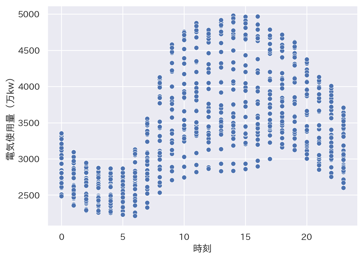

tempdata['daytime'] = (tempdata['time'] >= 9) & (tempdata['time'] <= 18)

tempdata['daytime'] = 1 * tempdata['daytime']
tempdata['elec100'] = tempdata['elec'] / 100
tempdata['time12'] = tempdata['time'] % 12
tempdata['ampm'] = np.where(tempdata['time'] < 12, "a.m.", 'p.m.')

4.3.2 重回帰分析

result = ols('elec ~ temp + daytime', data = tempdata).fit()

result.params

Intercept    -69.550278
temp         116.978245
daytime      555.442416
dtype: float64

result = ols('elec ~ temp + daytime + prec', data = tempdata).fit()

result.params

Intercept    -64.502521
temp         116.802353
daytime      556.147856
prec          -3.366077
dtype: float64

tempdata['sunday'] = (
    (tempdata['date'] == "2014/8/3") |
    (tempdata['date'] == "2014/8/10") |
    (tempdata['date'] == "2014/8/17") |
    (tempdata['date'] == "2014/8/24") |
    (tempdata['date'] == "2014/8/31")
)

tempdata['date'] = pd.to_datetime(tempdata['date'])

tempdata['sunday'] = 1 * (tempdata['date'].dt.day_name() == "Sunday")

tempdata['recess'] = 1 * (
    ("2014-08-11" <= tempdata['date']) & (tempdata['date'] <= "2014-08-16")
)

result = ols('elec ~ temp + daytime + prec + sunday + recess', data = tempdata).fit()

result.params

Intercept    179.070695
temp         113.477332
daytime      563.528357
prec          14.274994
sunday      -448.392059
recess      -438.230097
dtype: float64

print(179.07 + 113.48 * 28 + 563.53 * 1 + 14.27 * 0 - 448.39 * 0 - 438.23 * 0)

3920.04

sum(result.params * [1, 28, 1, 0, 0, 0])

3919.9643433699653

4.4 決定係数と回帰分析

4.4.2 決定係数の出力

result = ols('elec ~ temp + daytime + prec + sunday + recess', data = tempdata).fit()

print(result.summary())

                            OLS Regression Results                            
==============================================================================
Dep. Variable:                   elec   R-squared:                       0.733
Model:                            OLS   Adj. R-squared:                  0.731
Method:                 Least Squares   F-statistic:                     405.5
Date:                Wed, 05 Jun 2024   Prob (F-statistic):          6.82e-209
Time:                        18:20:19   Log-Likelihood:                -5452.9
No. Observations:                 744   AIC:                         1.092e+04
Df Residuals:                     738   BIC:                         1.095e+04
Df Model:                           5                                         
Covariance Type:            nonrobust                                         
==============================================================================
                 coef    std err          t      P>|t|      [0.025      0.975]
------------------------------------------------------------------------------
Intercept    179.0707    114.088      1.570      0.117     -44.906     403.047
temp         113.4773      4.193     27.066      0.000     105.247     121.708
daytime      563.5284     29.716     18.964      0.000     505.190     621.867
prec          14.2750     14.701      0.971      0.332     -14.586      43.136
sunday      -448.3921     38.125    -11.761      0.000    -523.238    -373.547
recess      -438.2301     35.199    -12.450      0.000    -507.331    -369.129
==============================================================================
Omnibus:                       18.794   Durbin-Watson:                   0.289
Prob(Omnibus):                  0.000   Jarque-Bera (JB):               12.050
Skew:                           0.169   Prob(JB):                      0.00242
Kurtosis:                       2.476   Cond. No.                         236.
==============================================================================

Notes:
[1] Standard Errors assume that the covariance matrix of the errors is correctly specified.

result = ols('elec ~ temp', data = tempdata).fit()

print(result.summary())

                            OLS Regression Results                            
==============================================================================
Dep. Variable:                   elec   R-squared:                       0.518
Model:                            OLS   Adj. R-squared:                  0.517
Method:                 Least Squares   F-statistic:                     797.9
Date:                Wed, 05 Jun 2024   Prob (F-statistic):          9.40e-120
Time:                        18:20:19   Log-Likelihood:                -5672.7
No. Observations:                 744   AIC:                         1.135e+04
Df Residuals:                     742   BIC:                         1.136e+04
Df Model:                           1                                         
Covariance Type:            nonrobust                                         
==============================================================================
                 coef    std err          t      P>|t|      [0.025      0.975]
------------------------------------------------------------------------------
Intercept   -614.2722    143.223     -4.289      0.000    -895.442    -333.102
temp         145.0303      5.134     28.246      0.000     134.950     155.110
==============================================================================
Omnibus:                      126.253   Durbin-Watson:                   0.095
Prob(Omnibus):                  0.000   Jarque-Bera (JB):               28.679
Skew:                          -0.040   Prob(JB):                     5.92e-07
Kurtosis:                       2.042   Cond. No.                         220.
==============================================================================

Notes:
[1] Standard Errors assume that the covariance matrix of the errors is correctly specified.

4.4.3 決定係数は「モデルの正しさ」を保証しない

np.random.seed(2022)

a = np.random.choice(list(range(1, 7)), size = 16,  replace = True)
b = np.random.choice(list(range(1, 7)), size = 16,  replace = True)
c = np.random.choice(list(range(1, 7)), size = 16,  replace = True)
d = np.random.choice(list(range(1, 7)), size = 16,  replace = True)
e = np.random.choice(list(range(1, 7)), size = 16,  replace = True)
f = np.random.choice(list(range(1, 7)), size = 16,  replace = True)
g = np.random.choice(list(range(1, 7)), size = 16,  replace = True)

mydata = pd.DataFrame(np.array([a, b, c, d, e, f, g]).transpose(), columns = ['a', 'b', 'c', 'd', 'e', 'f', 'g'])

print(ols('a ~ b + c + d + e + f + g', data = mydata).fit().summary())

                            OLS Regression Results                            
==============================================================================
Dep. Variable:                      a   R-squared:                       0.104
Model:                            OLS   Adj. R-squared:                 -0.493
Method:                 Least Squares   F-statistic:                    0.1748
Date:                Wed, 05 Jun 2024   Prob (F-statistic):              0.977
Time:                        18:20:19   Log-Likelihood:                -31.976
No. Observations:                  16   AIC:                             77.95
Df Residuals:                       9   BIC:                             83.36
Df Model:                           6                                         
Covariance Type:            nonrobust                                         
==============================================================================
                 coef    std err          t      P>|t|      [0.025      0.975]
------------------------------------------------------------------------------
Intercept      4.0021      4.667      0.858      0.413      -6.554      14.559
b              0.2341      0.399      0.587      0.571      -0.667       1.136
c              0.0051      0.406      0.012      0.990      -0.914       0.924
d              0.0703      0.401      0.175      0.865      -0.837       0.978
e              0.1139      0.377      0.302      0.769      -0.738       0.966
f             -0.3947      0.587     -0.673      0.518      -1.722       0.933
g             -0.3743      0.467     -0.801      0.444      -1.431       0.682
==============================================================================
Omnibus:                        2.883   Durbin-Watson:                   1.460
Prob(Omnibus):                  0.237   Jarque-Bera (JB):                1.350
Skew:                           0.341   Prob(JB):                        0.509
Kurtosis:                       1.751   Cond. No.                         69.6
==============================================================================

Notes:
[1] Standard Errors assume that the covariance matrix of the errors is correctly specified.

/Library/Frameworks/Python.framework/Versions/3.10/lib/python3.10/site-packages/scipy/stats/_stats_py.py:1736: UserWarning:

kurtosistest only valid for n>=20 ... continuing anyway, n=16

h = np.random.choice(list(range(1, 7)), size = 16,  replace = True)

mydata["h"] = h

print(ols('a ~ b + c + d + e + f + g + h', data = mydata).fit().summary())

                            OLS Regression Results                            
==============================================================================
Dep. Variable:                      a   R-squared:                       0.132
Model:                            OLS   Adj. R-squared:                 -0.627
Method:                 Least Squares   F-statistic:                    0.1745
Date:                Wed, 05 Jun 2024   Prob (F-statistic):              0.984
Time:                        18:20:19   Log-Likelihood:                -31.721
No. Observations:                  16   AIC:                             79.44
Df Residuals:                       8   BIC:                             85.62
Df Model:                           7                                         
Covariance Type:            nonrobust                                         
==============================================================================
                 coef    std err          t      P>|t|      [0.025      0.975]
------------------------------------------------------------------------------
Intercept      5.2407      5.445      0.963      0.364      -7.315      17.796
b              0.2238      0.416      0.537      0.606      -0.737       1.184
c              0.0078      0.424      0.018      0.986      -0.970       0.986
d              0.0113      0.435      0.026      0.980      -0.991       1.014
e              0.1094      0.393      0.278      0.788      -0.797       1.016
f             -0.2770      0.655     -0.423      0.683      -1.787       1.233
g             -0.3427      0.492     -0.697      0.505      -1.476       0.791
h             -0.3512      0.690     -0.509      0.624      -1.941       1.239
==============================================================================
Omnibus:                        1.901   Durbin-Watson:                   1.336
Prob(Omnibus):                  0.387   Jarque-Bera (JB):                1.382
Skew:                           0.528   Prob(JB):                        0.501
Kurtosis:                       2.022   Cond. No.                         85.8
==============================================================================

Notes:
[1] Standard Errors assume that the covariance matrix of the errors is correctly specified.

/Library/Frameworks/Python.framework/Versions/3.10/lib/python3.10/site-packages/scipy/stats/_stats_py.py:1736: UserWarning:

kurtosistest only valid for n>=20 ... continuing anyway, n=16

補足

tempdata = pd.read_csv('temperature_aug.csv')

result = ols('elec ~ temp', data = tempdata).fit()

ehat = result.resid

sum(ehat)

3.1377567211166024e-09

sum(tempdata['temp'] * ehat)

8.916094884625636e-08

4章 回帰分析の基礎

モジュールのインポート

4.1 回帰分析の考え方

4.1.4 数値例：気温と電力使用量

4.1.6 ノンパラメトリック回帰の実行

4.2 単回帰分析

4.2.1 ノンパラメトリック回帰の限界

4.2.4 Rによる線形回帰分析

4.3 重回帰分析

4.3.1 説明変数を追加する

4.3.2 重回帰分析

4.4 決定係数と回帰分析

4.4.2 決定係数の出力

4.4.3 決定係数は「モデルの正しさ」を保証しない

補足

4章回帰分析の基礎