第10章のStataコード
第10章 不連続回帰デザイン
10.2 条件付平均トリートメント効果 \(\tau\) の推定
10.2.1 条件付期待値が線形の場合
import delimited "exam_rdd.csv", case(preserve) clear

list in 1/4
+-------------------------------------+
| Y Z D Zc |
|-------------------------------------|
1. | 72.73265 57.01068 1 -2.989323 |
2. | 76.89065 75.34742 0 15.34742 |
3. | 51.04673 64.33642 0 4.336418 |
4. | 77.16946 73.30554 0 13.30554 |
+-------------------------------------+generate D = 0
replace D = 1 if Z < 60
replace D = . if missing(Z)
generate Zc = Z - 60
regress Y i.D##c.Zc Source | SS df MS Number of obs = 200
-------------+---------------------------------- F(3, 196) = 27.13
Model | 6787.05689 3 2262.3523 Prob > F = 0.0000
Residual | 16341.3052 196 83.3740063 R-squared = 0.2935
-------------+---------------------------------- Adj R-squared = 0.2826
Total | 23128.3621 199 116.222925 Root MSE = 9.1309
------------------------------------------------------------------------------
Y | Coefficient Std. err. t P>|t| [95% conf. interval]
-------------+----------------------------------------------------------------
1.D | 13.04019 2.03363 6.41 0.000 9.029581 17.05079
Zc | .8255922 .1154113 7.15 0.000 .5979848 1.0532
|
D#c.Zc |
1 | -.164973 .1674706 -0.99 0.326 -.4952487 .1653027
|
_cons | 60.06645 1.455575 41.27 0.000 57.19585 62.93705
------------------------------------------------------------------------------10.2.2 条件付期待値が非線形の場合
global bw 5

regress Y i.D if abs(Zc) <= $bw
Source | SS df MS Number of obs = 74
-------------+---------------------------------- F(1, 72) = 25.40
Model | 2045.40156 1 2045.40156 Prob > F = 0.0000
Residual | 5798.04804 72 80.5284451 R-squared = 0.2608
-------------+---------------------------------- Adj R-squared = 0.2505
Total | 7843.44961 73 107.444515 Root MSE = 8.9738
------------------------------------------------------------------------------
Y | Coefficient Std. err. t P>|t| [95% conf. interval]
-------------+----------------------------------------------------------------
1.D | 10.6559 2.114343 5.04 0.000 6.441033 14.87076
_cons | 62.07362 1.611736 38.51 0.000 58.86069 65.28656
------------------------------------------------------------------------------regress Y i.D##c.Zc if abs(Zc) <= $bw Source | SS df MS Number of obs = 74
-------------+---------------------------------- F(3, 70) = 8.44
Model | 2083.94121 3 694.647071 Prob > F = 0.0001
Residual | 5759.50839 70 82.2786913 R-squared = 0.2657
-------------+---------------------------------- Adj R-squared = 0.2342
Total | 7843.44961 73 107.444515 Root MSE = 9.0708
------------------------------------------------------------------------------
Y | Coefficient Std. err. t P>|t| [95% conf. interval]
-------------+----------------------------------------------------------------
1.D | 10.29327 4.689141 2.20 0.031 .9410765 19.64547
Zc | -.6093804 1.213381 -0.50 0.617 -3.029393 1.810632
|
D#c.Zc |
1 | 1.05658 1.548348 0.68 0.497 -2.031503 4.144663
|
_cons | 63.6814 3.592053 17.73 0.000 56.51727 70.84552
------------------------------------------------------------------------------Rによるデータ演習
import delimited "incumbency.csv", case(preserve) clear

list in 1/4
+----------------------+
| votesh~e margin |
|----------------------|
1. | .580962 .1048695 |
2. | .4610585 .1392521 |
3. | .5434108 -.0736019 |
4. | .5845801 .0868215 |
+----------------------+generate D = 0
replace D = 1 if margin >= 0
replace D = . if missing(margin)twoway scatter voteshare margin, ytitle("得票率") xtitle("前回の得票率 - 当落線")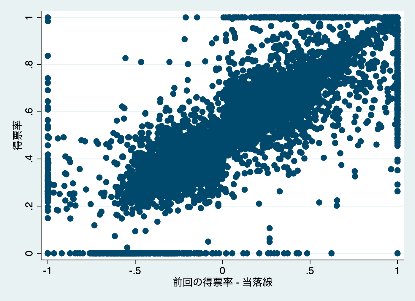
ssc install rddensity

rddensity margin, c(0)
Computing data-driven bandwidth selectors.
Point estimates and standard errors have been adjusted for repeated observations.
(Use option nomasspoints to suppress this adjustment.)
RD Manipulation test using local polynomial density estimation.
c = 0.000 | Left of c Right of c Number of obs = 6559
-------------------+---------------------- Model = unrestricted
Number of obs | 2740 3819 BW method = comb
Eff. Number of obs | 1297 1361 Kernel = triangular
Order est. (p) | 2 2 VCE method = jackknife
Order bias (q) | 3 3
BW est. (h) | 0.236 0.243
Running variable: margin.
------------------------------------------
Method | T P>|T|
-------------------+----------------------
Robust | 1.4240 0.1545
------------------------------------------
P-values of binomial tests. (H0: prob = .5)
-----------------------------------------------------
Window Lengtbw / 2 | <c >=c | P>|T|
-------------------+----------------------+----------
0.002 | 6 14 | 0.1153
0.003 | 14 21 | 0.3105
0.005 | 26 30 | 0.6889
0.006 | 33 42 | 0.3557
0.008 | 40 47 | 0.5203
0.009 | 45 50 | 0.6817
0.011 | 50 60 | 0.3909
0.012 | 57 67 | 0.4191
0.014 | 68 75 | 0.6160
0.015 | 75 84 | 0.5259
-----------------------------------------------------global bw 0.25
regress voteshare i.D##c.margin if abs(margin) <= $bw Source | SS df MS Number of obs = 2,764
-------------+---------------------------------- F(3, 2760) = 628.10
Model | 24.5646594 3 8.18821981 Prob > F = 0.0000
Residual | 35.9807376 2,760 .013036499 R-squared = 0.4057
-------------+---------------------------------- Adj R-squared = 0.4051
Total | 60.545397 2,763 .02191292 Root MSE = .11418
------------------------------------------------------------------------------
voteshare | Coefficient Std. err. t P>|t| [95% conf. interval]
-------------+----------------------------------------------------------------
1.D | .081653 .0084433 9.67 0.000 .0650971 .0982089
margin | .3665293 .0432142 8.48 0.000 .281794 .4512647
|
D#c.margin |
1 | .0848943 .0606704 1.40 0.162 -.0340697 .2038583
|
_cons | .4508738 .0060691 74.29 0.000 .4389735 .4627742
------------------------------------------------------------------------------global bw 0.05
regress voteshare i.D##c.margin if abs(margin) <= $bw Source | SS df MS Number of obs = 611
-------------+---------------------------------- F(3, 607) = 39.51
Model | 1.48124532 3 .493748439 Prob > F = 0.0000
Residual | 7.58534313 607 .012496447 R-squared = 0.1634
-------------+---------------------------------- Adj R-squared = 0.1592
Total | 9.06658845 610 .01486326 Root MSE = .11179
------------------------------------------------------------------------------
voteshare | Coefficient Std. err. t P>|t| [95% conf. interval]
-------------+----------------------------------------------------------------
1.D | .0453819 .0188994 2.40 0.017 .0082657 .0824982
margin | .9028807 .4810046 1.88 0.061 -.0417544 1.847516
|
D#c.margin |
1 | .109985 .6445108 0.17 0.865 -1.155757 1.375727
|
_cons | .4692386 .0139129 33.73 0.000 .4419153 .4965619
------------------------------------------------------------------------------postfile rdd bw betahat lci uci using rdd, replace
forvalues bw = 0.01(0.01)0.25 {
quietly regress voteshare i.D##c.margin if abs(margin) <= `bw'
matrix result = r(table)
post rdd (`bw' ) (result["b", "1.D"]) (result["ll", "1.D"]) (result["ul", "1.D"])
}
postclose rdd
preserve
use rdd, clear
twoway (rcap lci uci bw) (scatter betahat bw), yline(0, lpattern(dash)) legend(off) xtitle("バンド幅") ytitle("トリートメント効果の推定値")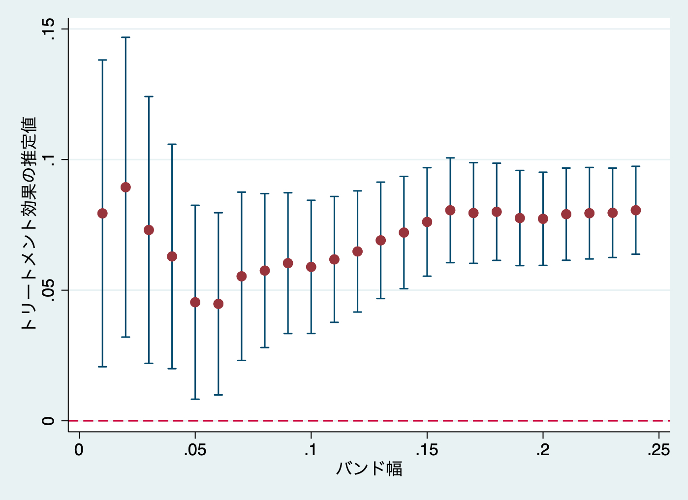
ssc install rdrobust

rdrobust voteshare margin, c(0) kernel(uniform)
Mass points detected in the running variable.
Sharp RD estimates using local polynomial regression.
Cutoff c = 0 | Left of c Right of c Number of obs = 6559
-------------------+---------------------- BW type = mserd
Number of obs | 2740 3819 Kernel = Uniform
Eff. Number of obs | 698 730 VCE method = NN
Order est. (p) | 1 1
Order bias (q) | 2 2
BW est. (h) | 0.120 0.120
BW bias (b) | 0.246 0.246
rho (h/b) | 0.489 0.489
Unique obs | 2606 3210
Outcome: voteshare. Running variable: margin.
--------------------------------------------------------------------------------
Method | Coef. Std. Err. z P>|z| [95% Conf. Interval]
-------------------+------------------------------------------------------------
Conventional | .06483 .01124 5.7693 0.000 .042807 .086857
Robust | - - 4.8063 0.000 .035954 .085468
--------------------------------------------------------------------------------
Estimates adjusted for mass points in the running variable.