第9章のStataコード

第9章マッチング法

サンプルデータ

wage_training.csv：研修と賃金に関する架空データ．

Rによるデータ演習

import delimited "wage_training.csv", case(preserve) clear 

list in 1/4

     +-------------------------------------------+
     | wagea   D   years   wageb   educ   female |
     |-------------------------------------------|
  1. |    19   1       4      18     17        1 |
  2. |    27   0      22      27     13        0 |
  3. |    20   1       2      18     15        1 |
  4. |    36   1      14      34     14        1 |
     +-------------------------------------------+

summarize wagea if D == 1
local mean_treated = r(mean)

    Variable |        Obs        Mean    Std. dev.       Min        Max
-------------+---------------------------------------------------------
       wagea |        238    25.71849    4.542411         19         36

summarize wagea if D == 0
local mean_treated = r(mean)

    Variable |        Obs        Mean    Std. dev.       Min        Max
-------------+---------------------------------------------------------
       wagea |        562    26.84698    5.613652         18         40

display `mean_treated' - `mean_controlled'

-1.1284877

cor Y years wageb

             |        D    years    wageb
-------------+---------------------------
           D |   1.0000
       years |  -0.1908   1.0000
       wageb |  -0.1839   0.7772   1.0000

teffects nnmatch (wagea years wageb) (D), atet metric(ivariance)

Treatment-effects estimation                   Number of obs      =        800
Estimator      : nearest-neighbor matching     Matches: requested =          1
Outcome model  : matching                                     min =          1
Distance metric: ivariance                                    max =         14
------------------------------------------------------------------------------
             |              AI robust
       wagea | Coefficient  std. err.      z    P>|z|     [95% conf. interval]
-------------+----------------------------------------------------------------
ATET         |
           D |
   (1 vs 0)  |   1.047404   .0411316    25.46   0.000     .9667875     1.12802
------------------------------------------------------------------------------

tebalance summarize years wageb

(refitting the model using the generate() option)

Covariate balance summary

                         Raw      Matched
-----------------------------------------
Number of obs =          800          476
Treated obs   =          238          238
Control obs   =          562          238
-----------------------------------------

-----------------------------------------------------------------
                |Standardized differences          Variance ratio
                |        Raw     Matched           Raw    Matched
----------------+------------------------------------------------
          years |  -.4422582    .0060473      .6556135   1.020168
          wageb |  -.4246649   -.0006091      .6733798   .9989335
-----------------------------------------------------------------

quietly teffects nnmatch (wagea years wageb educ female) (D), atet metric(ivariance)
tebalance summarize years wageb educ female
clear
svmat double r(table), name(balance_summary)
rename balance_summary1 original_std_dif
rename balance_summary2 matched_std_dif
generate abs_original_std_dif = abs(original_std_dif)
generate abs_matched_std_dif = abs(matched_std_dif)
generate covariate = _n
local covariate 1 "years" 2 "wageb" 3 "educ" 4 "female"
label define covariate `covariate'
label values covariate covariate
twoway (scatter covariate abs_original_std_dif) (scatter covariate abs_matched_std_dif), xline(0.1) ylabel(`covariate', angle(0)) ytitle("") legend(label(1 "Original")) legend(label(2 "Matched"))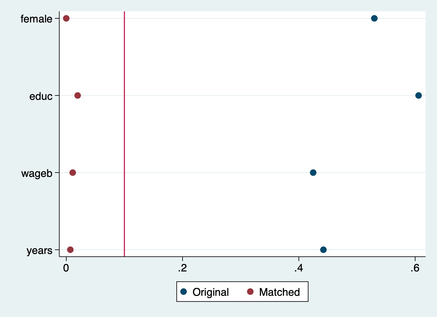

標準化平均差についての補足

RのMatchItパッケージでは，ATTを推定する場合，標準化平均差（standardized mean difference）を次の定義によって計算します¹．

\[ \text{SMD}^\text{R} = \frac{\hat{\mu}_T - \hat{\mu}_C}{\hat{\sigma}_T}. \]

ただし，\(\hat{\mu}_T\)はトリートメントグループにおける標本平均，\(\hat{\mu}_C\)はコントロールグループにおける標本平均，\(\hat{\sigma}_T\)はトリートメントグループにおける標準偏差を表します．対して，Stataのtebalanceは，ATTを推定する場合，標準化平均差を次の定義によって計算します²．

\[ \text{SMD}^\text{Stata} = \frac{\hat{\mu}_T - \hat{\mu}_C}{\sqrt{(\hat{\sigma}_T^2 + \hat{\sigma}_C^2)/2}}. \]

したがって，マッチング前の標準化平均差の値がRとStataとで異なっています．

脚注

参照：https://kosukeimai.github.io/MatchIt/reference/summary.matchit.html ↩︎
参照：Stata Treatment-Effects Reference Manual: Potential Outcomes/Counterfactual Outcomes Release 17, p.216.(https://www.stata.com/manuals/te.pdf)↩︎

第9章 マッチング法

Rによるデータ演習

標準化平均差についての補足

脚注

第9章マッチング法